How to Use FaceIt GUI

Open Data to Process

To analyze mouse face motion data, navigate to the File tab in the menu bar and select one of the following options:

• Folder — open a .npy image series (Ctrl + N)

• File — open a video file (Ctrl + V)

Once selected, the images or video frames will be displayed in the GUI for analysis.

—

Analyse Pupil

To begin pupil tracking, use the Pupil ROI button in the ROI Tools section to define the eyeball region. You can adjust the position of the ROI by dragging it, or resize it by clicking and dragging the blue square at its corner.

After selecting and adjusting the Eyeball ROI, you can use the Eraser option to remove pixels from the surrounding eye region. This ensures that these pixels are excluded from further analysis. The size of the eraser can be customized in the settings window.

After selecting and adjusting the eyeball ROI, use the Eraser option to remove unwanted pixels around the eye region. This ensures that these pixels are excluded from further analysis. You can customize the eraser size in the Settings window.

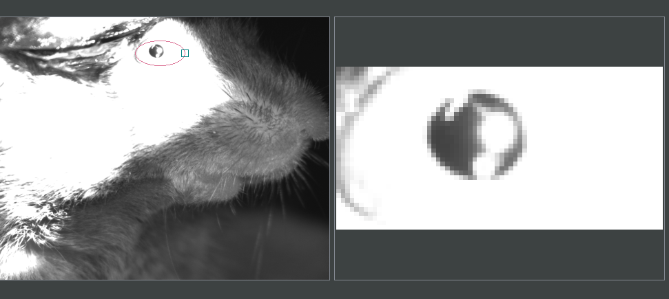
Figure: Example of eyeball ROI selection.

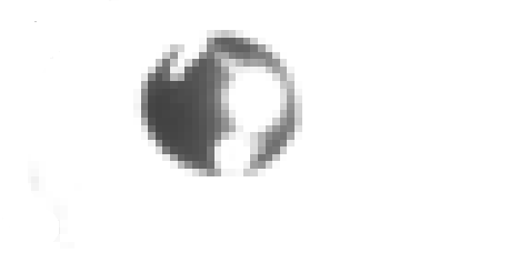
Figure: Erasing pixels from the surrounding eye region.

Important

Avoid erasing regions that the pupil might cross.

—

Pupil Area Visualization Modes

FaceIt provides two visualization modes for the pupil area:

• Normal preview — continuous, unthresholded pupil area trace.

• Binary preview — pupil area estimated from a thresholded (binary) mask.

Toggling the View

Use the Show Binary checkbox to switch between visualization modes.

Example Views

Below are examples of the two visualization modes displayed side by side:

Normal preview

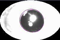
Binary preview

—

Binarization methods

You can choose how the binary mask is created. Two methods are available:

• Global (constant) binarization Applies a single threshold to the whole image.

• Adaptive binarization Computes a local threshold per neighborhood (robust to uneven illumination).

Selecting the method

By default, Adaptive binarization is used.

To switch methods, use the Constant Binary checkbox:

• Unchecked (default) → Adaptive binarization.

• Checked → Global (constant) binarization.

Figure: Threshold slider active in Global (Constant) mode.

When Constant Binary is checked, a threshold slider becomes active so you can set the global threshold used for the constant method.

Note

• In Adaptive mode, the global threshold slider is disabled; instead, tune Block size and C under Adaptive thresholding settings.

• In Constant mode, adjust the threshold slider to control the binary mask.

Parameters

• Global (constant):

  • Binary threshold: the global threshold value applied to all pixels.

• Adaptive:

  • Block size: window size for local statistics (larger → smoother, less detail).

  • C: constant subtracted from the local mean/weighted mean (higher C → stricter threshold).

When to use which

• Use Global when lighting is uniform and the pupil/eyeball contrast is stable.

• Use Adaptive when lighting is uneven, there are vignetting, or contrast varies across the frame.

Reflection Correction

Bright corneal reflections can fragment the pupil mask and bias ellipse fitting. FaceIt handles reflections in two ways:

• Automatic detection + inpainting (available only with Adaptive binarization; default)

• Manual reflection ellipses (available with Adaptive and Constant/Global)

Defaults

• The default Binarization method is Adaptive.

• In Adaptive mode, the pipeline applies automatic reflection detection + inpainting unless you provide manual ellipses.

Behavior by Binarization Method

Mode	Auto detect + inpaint	Manual ellipses
Adaptive	Yes (default)	Inpaint using ellipses
Constant / Global	No	Overlap fix (no inpainting)

How it works

Automatic (Adaptive only)

1. Detect bright regions using a percentile threshold controlled by Reflect br; filter by area/circularity; dilate proportionally to glare size.

2. Inpaint the detected mask (TELEA) to remove glare before adaptive thresholding.

Manual ellipses (both modes)

• Adaptive: skip auto-detect and inpaint directly using the provided ellipses.

• Constant/Global: after thresholding/clustering, apply an overlap fix—pixels where the fitted pupil ellipse overlaps a reflection ellipse are restored to the pupil mask (no inpainting).

Controls & parameters

• Binarization method - Adaptive (default): uses Block size and C (subtractive constant). - Constant/Global: uses one Binary threshold.

• Reflect br (slider, Adaptive only): sets the brightness percentile for automatic detection (higher → stricter, fewer pixels marked as reflections).

• Manual reflection ellipses (optional): user-specified ellipse masks used as above.

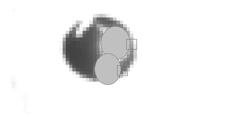
Adding manual reflection cover to the pupil.

Light Adjustment

Uneven illumination and low contrast can break the pupil mask. FaceIt provides two complementary tools to precondition frames before binarization:

• Uniform Image Adjustment — applies the same saturation and contrast across the entire image.

• Gradual Image Adjustment — applies a spatial brightness/saturation gradient to compensate for vignetting or directional lighting.

At a Glance

Tool	What it fixes	Typical use
Uniform	Low contrast overall	Quick global boost for dark ROI
Gradual	Uneven lighting/vignet.	Brighten one side or center edges

Uniform Image Adjustment

Enable with the Uniform Image Adjustments checkbox.

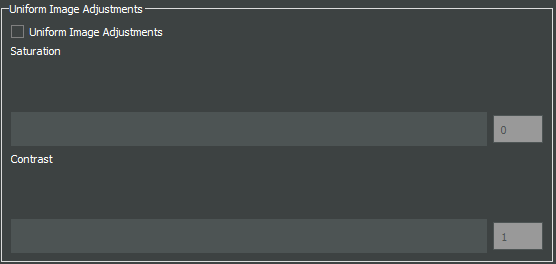
Figure: Uniform Image adjustment panel

Controls

• Saturation: percentage change to color saturation and value (brightness) uniformly.

• Contrast: multiplies contrast uniformly (e.g., 1.3 = +30%).

Behavior

Internally, images are converted to HSV. The S and V channels are scaled by the selected Saturation, then a simple contrast gain is applied on the BGR image.

When to use

• The whole ROI is too flat/dim, but illumination is roughly uniform.

• You want a quick global boost before trying more advanced correction.

Gradual Image Adjustment

Enable with the Gradual Image Adjustments checkbox.

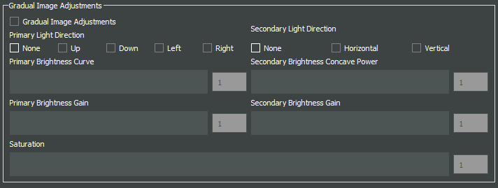
Figure: Uniform Image adjustment panel

This mode builds a brightness weight mask (a 2-D gradient) and multiplies it with the image brightness. Optionally, it can also adjust saturation non-uniformly.

Primary controls

• Primary Light Direction (radio buttons): Up, Down, Left, Right Chooses the direction along which brightness increases.

• Primary Brightness Curve: curvature of the gradient (≥ 1). Higher values make the ramp more curved (stronger bias at the bright end).

• Primary Brightness Gain: final multiplicative gain at the bright end (≥ 1).

Secondary controls

• Secondary Light Direction: None, Horizontal, Vertical Adds a symmetric concave gain (brighter toward edges) along the chosen axis.

• Secondary Brightness Concave Power: shape of the concave curve (≥ 1). Higher = steeper towards edges.

• Secondary Brightness Gain: how much the edges are boosted (≥ 1).

• Saturation: optional multiplicative factor for saturation in Gradual mode.

Behavior

• Builds a primary directional mask (linear ramp raised to Primary Brightness Curve).

• Optionally multiplies a symmetric concave mask (edges brighter) controlled by Secondary settings.

• Multiplies the HSV V channel by the combined mask; clamps into [0, 255].

• If Saturation is given, scales the HSV S channel as well.

Relation to binarization

• Both Uniform and Gradual adjustments are applied before binarization (Adaptive or Constant). The goal is to present a cleaner, more separable histogram to the thresholding stage.

• For Adaptive binarization, Gradual adjustment often reduces the load on Block size and C by flattening large-scale illumination differences.

• For Constant/Global binarization, Gradual adjustment helps meet a single threshold across the ROI.

Clustering (Choosing the Pupil Blob)

After binarization, FaceIt selects the pupil region from the foreground mask. You can choose a method in:

Options & Threshold → Clustering Method

Available methods:

• Simple Contour (default)

• DBSCAN

• Watershed

Figure: Clustring Methods

Default

Clustering Method: Simple Contour (with filtering enabled)

Output is the convex hull of the selected blob (fills small holes before ellipse fit).

Simple Contour

Algorithm:

1. Apply cv2.findContours on the binary mask.

2. (Optional) Filter contours by width, aspect ratio (W/H), and area.

3. Keep the largest remaining contour.

4. Draw and fill its convex hull.

Pros

• Fast and reliable when the pupil is already one blob.

Notes

• If the pupil breaks into several islands (fir example because of light reflection), consider DBSCAN.

DBSCAN

Algorithm:

1. Take coordinates of all non-zero pixels (foreground).

2. Cluster with DBSCAN (eps = mnd, min_samples = 1).

3. For each cluster, compute its bounding box and optionally filter out : - width > 80% of image width - aspect ratio W/H > 2

4. Select the largest valid cluster and fill its convex hull.

Pros

• Handles fragmented masks produced by glare removal or noise.

Tip

Note: MND applies only when using the DBSCAN clustering method.

You can change MND directly from the Settings window.

• Increase ``MND`` if the pupil mask is broken into too many small islands. A higher value makes DBSCAN merge nearby fragments into one larger cluster.

• Decrease ``MND`` if the algorithm merges too much and includes unwanted dark areas or noise. A smaller value keeps clusters more separated.

Quick Comparison

Analyse whisker pad

To analyse Whisker pad motion energy you can start by defining your region of interest using Face ROI bottom in the ROI tools section. check whisker pad checkbox and click on the process bottom. After the analysis is complete, a whisker pad motion energy plot will be displayed on the GUI. If grooming activity is present in your data, you can easily interpolate the grooming segments by setting a threshold on the y-axis of the motion energy plot. To do this, click on Define Grooming Threshold and select the area where you want to remove activity above the specified level. A new plot, with the grooming segments interpolated, will then be displayed.

Process data

Once the Pupil and Face (Whisker Pad) ROIs are selected and adjusted, you can start processing the data by checking the corresponding boxes under Options & Threshold and pressing the Process button.

• Check Whisker Pad to process face motion (motion energy analysis).

• Check Pupil to process pupil dilation and related parameters.

Only the ROIs with their checkboxes enabled will be processed. If an ROI checkbox is not selected, that data will be skipped during processing.

Data visualization in the GUI

After processing is finished, the computed signals are automatically displayed in the main GUI window for quick inspection.

The visualization area is divided into two main plots:

• Top panel (orange) — Face motion Displays the motion energy trace.

• Bottom panel (green) — Pupil Displays the raw or filtered pupil area trace. Vertical ticks mark detected saccades (big ye movement).

Both panels share a common x-axis, representing frame number.

Figure: Data visualization in the GUI

Navigation and interaction

• A blue vertical line indicates the current frame. It moves dynamically as you slide through frames with the bottom slider.

• The horizontal slider allows continuous browsing through frames.

• You can jump to a specific frame by entering its number in the small box next to the slider and pressing Enter.

Post processing

After the main processing finishes, FaceIt provides optional post-processing tools you can apply to clean signals and flag artifacts. All actions are undoable.

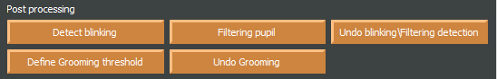
Figure: Post Processing Panel

Detect blinking

Idea:

Identify blinks using (a) geometry changes (width/height ratio) and (b) large pupil drops; replace blink segments by interpolation and mask saccades at the same indices.

Algorithm (short):

1. Compute ratio = width / height.

2. Detect candidate blink indices from: - ratio using a robust threshold, - pupil area using a robust threshold.

3. Union the indices, bound them to signal length, and mask saccades (set to NaN at blink indices).

4. Interpolate the pupil trace across those indices.

API.

ids = process_handler.detect_blinking(
    pupil=pupil_area, width=width, height=height,
    x_saccade=X_sacc, y_saccade=Y_sacc
)
# → Updates: app.interpolated_pupil, X/Y_saccade_updated

Note

• Because Detect blinking relies on the geometry of the detected cluster, the option “Filter Cluster” (in Options & Threshold → Clustering Method) should be unchecked. Filtering can smooth or alter the cluster’s shape, reducing blink detection accuracy.

• This method performs best when using a global binarization method rather than an adaptive one.

Filtering pupil (Hampel)

Idea:

Robust outlier removal on the pupil time series using a Hampel filter (rolling median ± k·MAD). Outlier samples are treated as blinks: saccades are masked at those indices and the pupil is interpolated.

Parameters.

• win: half-window size for rolling statistics.

• k: outlier threshold multiplier (default ≈ 3.0).

API.

ids = process_handler.Pupil_Filtering(
    pupil=pupil_area,
    x_saccade=X_sacc, y_saccade=Y_sacc,
    win=15, k=3.0
)
# → Updates: app.interpolated_pupil, X/Y_saccade_updated

Grooming threshold

Idea:

When animals groom, the face-motion signal shows large bursts. Define a threshold to clip those bursts while keeping baseline dynamics. Clipped indices are returned for reference.

API.

facemotion_clean, groom_ids, thr = process_handler.remove_grooming(
    grooming_thr=threshold_value,
    facemotion=facemotion_trace
)
# → Also stores: app.facemotion_without_grooming

Undo actions

• Undo blinking/Filtering detection restores the pupil trace and saccades to their pre-blink/pre-filter state.

• Undo Grooming restores the original face-motion signal (before clipping).

Saving data

When you click the Save button, the processing results are automatically stored in .npz files. To save the data in .nwb format, ensure you select the Save NWB checkbox before saving.

In addition, several visualization images (.png) are automatically saved in the same directory to provide a quick overview of the processed results.

To better understand what is contained in the saved files, refer to the Output section of this documentation.